Mexico City Housing Prices
Data Analysis · Data Cleaning · Linear Regression
This project analyzes residential listings in Mexico City to understand price levels, size distributions, and spatial patterns. The workflow performs rigorous data cleaning, exploratory visualization, KPI aggregation by borough, geospatial mapping, and a baseline modeling step to explain prices from property attributes.
Objective
Build a clear, reliable view of the housing market in Mexico City by cleaning raw listings, removing unrealistic observations and outliers, summarizing key indicators (USD/m², price levels, stock), and modeling log-prices using structural features and location.
Dataset
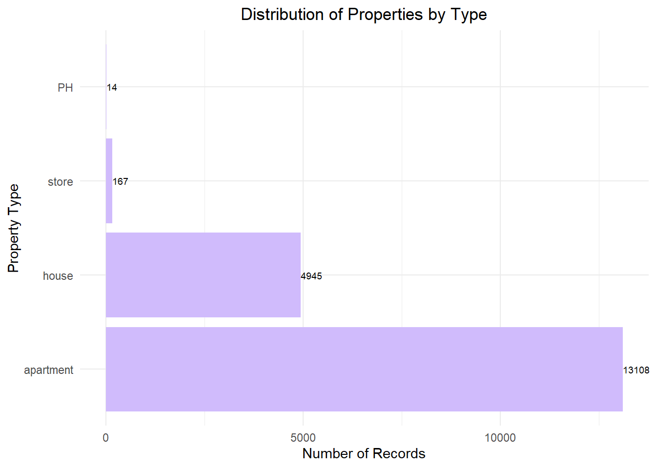
- CSV of listings with columns such as property_type, places (borough), price_usd, surface_total_in_m2, surface_covered_in_m2, price_usd_per_m2, lat, lon.
- Initial shape inspection, summary statistics, and column pruning (e.g., removing
lat.lon, currency fields, and derived duplicates).
Tools and Technologies
- R (tidyverse, janitor, dplyr, ggplot2, patchwork)
- Data quality & cleaning: outlier treatment with IQR, logical filters, duplicate and NA checks
- Visualization: histograms, boxplots (log scales), borough rankings
- Geospatial: leaflet (CartoDB tiles, circle markers, legends)
- Modeling & summaries: broom, base
lm()for log-price regression
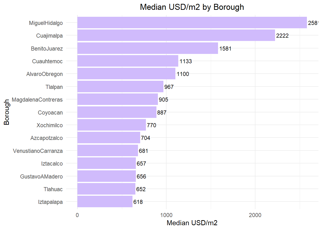
KPI Highlights by Borough
- Highest USD/m²: Miguel Hidalgo (~2,580 USD/m²) and Cuajimalpa (~2,220 USD/m²), reflecting premium zones like Polanco and Santa Fe.
- Second tier: Benito Juárez (~1,580), Cuauhtémoc (~1,130), Álvaro Obregón (~1,100) with strong central demand.
- Mid-range: Coyoacán, Magdalena Contreras, Tlalpan show moderate medians with wider dispersion.
- More affordable: Iztapalapa, Tláhuac, Gustavo A. Madero around ~600–660 USD/m².
Modeling
A linear model on log-price (log(price_usd)) with predictors log(surface_total_in_m2), covered_ratio, property_type, and places quantifies elasticities and location effects.
Size has a positive elasticity with diminishing returns (log–log), while borough and property type explain substantial residual variation.
Results
- Cleaning reduced extreme skew: after removing unrealistic sizes, duplicate rows, and inconsistent price–size pairs, histograms and boxplots present compact, interpretable distributions.
- Outlier review flagged ~130 contradictory cases; excluding them aligns USD/m² distributions and clarifies borough rankings.
- Clear spatial segmentation emerges: premium corridors in the west/center vs. more affordable eastern and southern boroughs.
Key Learnings
- Domain-aware rules (e.g., covered ≤ total, practical size floors) are essential before statistical outliering.
- Log-scaling is crucial for heavy-tailed real estate variables (price, area, USD/m²) to reveal structure.
- Borough fixed effects matter: location shifts dominate after controlling for size and coverage.
- Interactive maps accelerate anomaly detection and geocleaning versus charts alone.